Preprint · August 2026 Scientific machine learning
Discretization and Statistical Consistency of Functional Flow Matching
Changing the grid changes the information. When do finite observations recover the same function-space flow?
Georgia Institute of Technology
arXiv preprint · arXiv:2608.04531
Projection and conditioning are different operations. Their relationship is the missing sensor limit.
Abstract
Functional flow matching is posed on distributions of functions but implemented from finitely many coefficients or point values. Under scattered or adaptive refinement, the resulting conditioning sigma-algebras need not be nested, so martingale convergence does not justify the sensor limit. We prove strong L² convergence of finite conditional velocity targets for every strongly consistent sequence of finite-rank reconstructions, with quantitative bounds for orthogonal projections and a point-sensor extension through a regularity space. For learned flows, coupling directly to a population superposition path yields an end-to-end Wasserstein bound without assuming uniqueness of the population finite-dimensional ODE. We verify sensor-independent constants for a normalized quadrature neural operator, including globally Lipschitz activations through an explicit magnitude recurrence. A noncommuting trace-class Gaussian example gives boundary multiplier 0 under projected restriction and 0.72 under exact conditioning. A spatial regularity–cubature certificate closes the operator-realization term, a Bernstein argument gives an Õ(n⁻¹) excess-risk term for fixed model dimension and envelopes, and an exactly realizable clipped Gaussian scaling specialization yields an explicit end-to-end rate.
The method
Functional flow matching defines a velocity on a distribution of functions, while implementations observe finitely many coefficients or point values. With scattered, remeshed, or adaptive observations, successive information sets need not be nested. Strong convergence of reconstructed states alone does not make a martingale argument available.
Theorem 7: strongly consistent finite-rank reconstruction; no nested observation sigma-algebras. The norm averages over time and probability.
- 01
Prove the conditional-target limit
Write the finite target as the reconstruction operator applied to a conditional expectation of the continuum velocity. Approximate that velocity by bounded continuous functions of time and state, then use consistency of reconstructed observations. Theorem 7 proves strong L² convergence without nested sigma-algebras.
- 02
Control the implemented operator and learning risk
Verify sensor-independent constants for a normalized quadrature neural operator, including ReLU, GeLU, and SiLU through an explicit magnitude recurrence. A regularity–cubature certificate controls realization error; a Bernstein argument yields a fast excess-risk term for fixed model dimension and envelopes.
- 03
Propagate risk to the generated law
Couple the learned ODE directly to a population superposition path. Stability is imposed on the learned field, so population finite-dimensional ODE uniqueness is unnecessary for the generated-law bound. Add numerical integration, reconstruction, and endpoint errors explicitly.
Under the paper’s learned-field stability, statistical, and coupled-solver assumptions. Approximation, target refinement, and operator realization enter through the risk certificate.
Projection or conditioning?
Evaluate the exact formulas from Proposition 30 on the mixed observed direction gₘ = (e₂ₘ₋₁ + e₂ₘ)/√2. These are analytic coefficients, not learned neural-network predictions.
(k₊ + k₋) / 2
(D₊ + D₋) / (Q₊ + Q₋)
At the paper’s t = 0.5 and ratios 4 and 1/4, the multipliers are 0 and 0.72. With equal ratios they coincide. The local coefficient gap does not contradict global consistency: the affected direction moves into a vanishing trace-class tail.
Theoretical results & numerical check
The main results are consistency theorems and a composed error bound. A trace-class Gaussian example makes the distinction between projection and conditioning explicit. Its finite-sample check fits one boundary multiplier over 200 independent repetitions at each sample size; it is not a learned-operator benchmark.
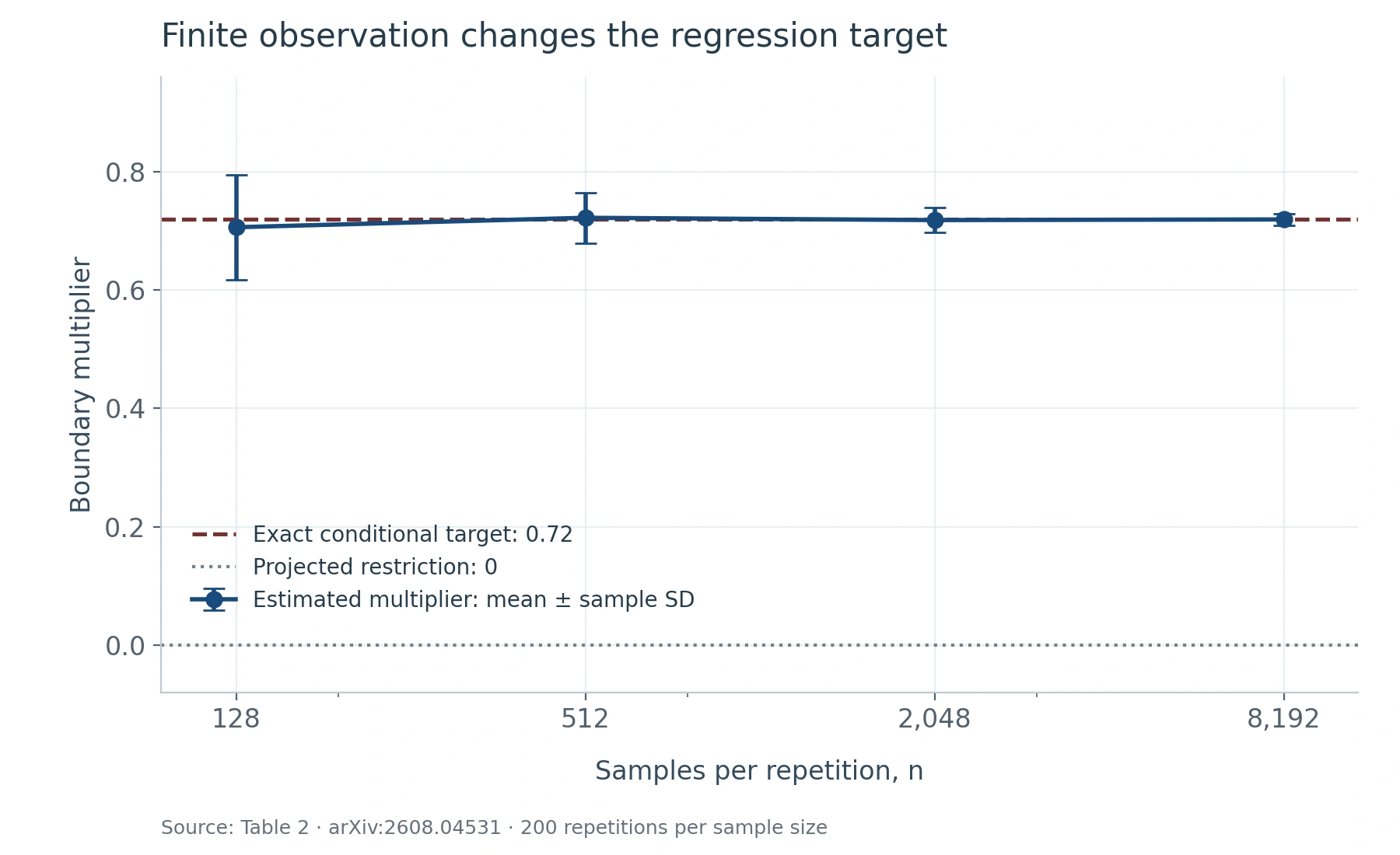
Finite observations change the conditional target
Plotted from Table 2. The estimated boundary multiplier approaches the exact conditional value 0.72, whereas projected restriction gives 0. Points are reported means; error bars are sample standard deviations over 200 repetitions, not confidence intervals.
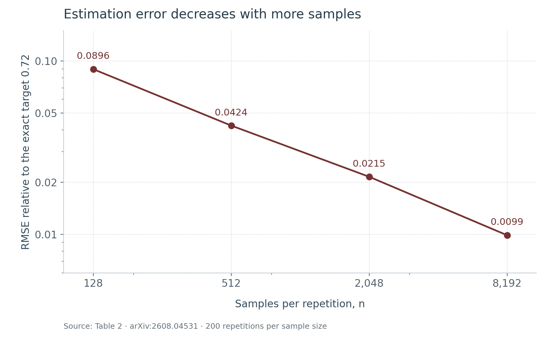
The finite-sample check resolves the conditioning gap
Reported RMSE decreases from 0.0896 at n = 128 to 0.0099 at n = 8192. These values measure estimation error relative to 0.72; they do not measure the full generated-law error or establish a learned neural operator’s convergence rate.
From finite sensors to a generated probability law
| Result | What is established | Conditions and scope |
|---|---|---|
| Theorem 7 | Strong L² convergence of finite conditional targets | Strongly consistent, uniformly bounded finite-rank reconstructions; observations need not be nested |
| Theorem 17 | Sensor-independent operator constants | The specified normalized quadrature architecture and norm bridge |
| Theorem 18 | Õ(n⁻¹) excess-risk term | Fixed model dimension and envelopes; approximation and optimization terms remain |
| Proposition 21 | Operator-realization consistency | Spatial regularity, stable reconstruction, and W₁ cubature control |
| Theorem 26 | End-to-end W₂ error decomposition | Learned-field stability, a risk certificate, and a coupled solver guarantee |
| Corollary 33 | O((log n)/√n) generated-law rate | Exactly realizable clipped Gaussian scaling model and the stated joint schedule |
The results have distinct assumptions. The fast excess-risk term and the generated-law rate are different quantities; neither is an unconditional guarantee for every flow-matching architecture or refinement sequence.
What the results mean
An order-one local discrepancy can coexist with convergence
At t = 1/2, with endpoint variance ratios 4 and 1/4, the two continuum multipliers are 1.2 and −1.2. Their projected average is 0, but conditioning on the mixed observed direction gives 0.72. As refinement moves that boundary direction into the trace-class tail, its contribution to the global L² error still vanishes.
Three meanings of resolution invariance
Information refinement reconstructs the same random function. Mesh transfer evaluates an operator using a new quadrature. Frequency extrapolation asks for components absent from the observations and hypothesis class. The paper supplies certificates for the first two under stated assumptions; it does not turn them into a guarantee of the third.
A stability boundary is not a convergence failure
The paper also constructs a globally 1-Lipschitz continuum velocity whose finite conditional targets have no mesh-uniform Lipschitz envelope. Its finite flows nevertheless equal the projected continuum flow. The example limits a sufficient stability assumption, rather than showing that discretized flows must fail to converge.
Scope and limitations
The results require controlled reconstruction, operator realization, learning envelopes, and learned-field stability. Point sensors require a regularity space and stable reconstruction. The fast excess-risk term assumes fixed model dimension and envelopes; the explicit end-to-end rate concerns an exactly realizable clipped Gaussian scaling model. The theory does not establish unseen-frequency recovery, infinite-dimensional likelihoods, or a mesh-uniform certificate for standard FNOs. The numerical check isolates the conditioning mechanism rather than benchmarking a learned operator.
Relevant to consistency of function-space generative models, functional flow matching on changing grids, scattered and adaptive sensors, mesh-uniform neural operator analysis, and Wasserstein guarantees for learned probability flows.
- Functional flow matching
- Discretization consistency
- Nonnested observations
- Function-space generative models
- Wasserstein error bounds
- Neural operator learning theory
Citation & resources
Lennon J. Shikhman. Discretization and Statistical Consistency of Functional Flow Matching. arXiv preprint · arXiv:2608.04531, 2026.
arXiv:2608.04531
@article{shikhman2026discretization,
  title={Discretization and Statistical Consistency of Functional Flow Matching},
  author={Shikhman, Lennon J.},
  journal={arXiv preprint arXiv:2608.04531},
  year={2026},
  eprint={2608.04531},
  archivePrefix={arXiv},
  primaryClass={cs.LG},
  url={https://arxiv.org/abs/2608.04531}
}
The numerical plots use the values reported in Table 2 of the paper; no new empirical results are introduced. The Gaussian explorer evaluates the analytic formulas in Proposition 30.